Article
From Waves to Vectors: The Engineer's Guide to Audio for AI (Part 1)

From Waves to Vectors: The Engineer's Guide to Audio for AI
As software engineers, we are comfortable with discrete data: strings, integers, JSON objects. We like our data deterministic and finite.
Audio is none of those things.
Audio is continuous, chaotic, and physically bound by time. Before we can feed audio into any AI model, we need to understand what sound actually is - how it behaves in the physical world, and how engineers have learned to capture, digitize, and transform it.
In this deep dive (Part 1 of our Speech AI series), we will strip away the academic jargon of signal processing and look at audio through the lens of Data Engineering. We will trace the transformation of a spoken word from air pressure variations into the 2D "image" that AI models can consume.
🌊 The Physics of Sound: What Are We Actually Capturing?
Before we touch any code, let's understand the physical phenomenon we're dealing with. Sound is not magic - it's mechanical.
How Sound Travels
When you speak, your vocal cords vibrate. These vibrations push against air molecules, creating a chain reaction of compressions and rarefactions (areas of high and low pressure) that propagate outward like ripples in a pond.
 Figure 1: Sound as a physical phenomenon - pressure waves traveling through air from source to receiver. [Source: Wikimedia Commons][1]
This is a longitudinal wave - the air molecules don't travel from your mouth to someone's ear; they oscillate back and forth, passing energy along. Think of it like a stadium wave: people don't run across the stadium, they just stand and sit in sequence.
The Two Dimensions of Sound
Sound consists of pressure waves moving through the air. To digitize this, we measure two fundamental properties:
1. Amplitude (The Y-Axis): Loudness
Amplitude measures how much the air pressure changes from its resting state.
- Physical Reality: Large pressure changes = molecules pushed harder = louder sound
- Measurement: Typically measured in decibels (dB), a logarithmic scale
- In Code: It's the value of your float (e.g., 0.0 is silence, 1.0/-1.0 is maximum volume)
- Fun Fact: A whisper is ~30 dB, conversation is ~60 dB, a rock concert is ~110 dB. Because dB is logarithmic, every 10 dB increase sounds roughly twice as loud.
2. Frequency (The X-Axis Pattern): Pitch
Frequency measures how fast the pressure oscillates.
- Physical Reality: Fast vibrations = high pitch (think violin), slow vibrations = low pitch (think bass drum)
- Unit: Hertz (Hz) = cycles per second
- Human Range: We hear approximately 20 Hz to 20,000 Hz
- Speech Range: Human voice fundamental frequencies typically fall between 85 Hz (deep male voice) and 300 Hz (high female voice), with harmonics extending higher

Complex Sounds: Why Instruments Sound Different
Real sounds aren't simple waves. When you pluck a guitar string, you don't just get one frequency - you get the main note (called the fundamental) plus a bunch of quieter "echo" frequencies called harmonics.
This is why a piano and a guitar playing the same note sound different. They share the same main note, but their mix of harmonics is different. This unique "fingerprint" is called timbre (pronounced "TAM-ber").
Human speech is incredibly complex - each vowel sound is a unique mix of frequencies, and consonants add bursts of noise and rapid changes.
🎚️ Capturing the Continuous: Sampling Rate & Bit Depth
Here's the fundamental challenge: computers can only store discrete values, but sound waves are continuous. How do we bridge this gap?
The answer is sampling - we take regular "snapshots" of the sound wave.
Sampling Rate: The "Frame Rate" of Audio
Just like video has Frame Rate (30 fps or 60 fps), audio has Sampling Rate. It defines how many times per second the computer measures the sound pressure.
| Format | Sampling Rate | Use Case |
|---|---|---|
| Telephone | 8,000 Hz | Voice only, bandwidth limited |
| Speech AI | 16,000 Hz | Speech recognition, optimal for voice |
| CD Quality | 44,100 Hz | Music, full frequency range |
| Professional | 96,000+ Hz | Studio recording, archival |
The Nyquist-Shannon Theorem: Why These Numbers?
This is one of the most important theorems in signal processing. It states:
To perfectly reconstruct a continuous signal, you must sample at at least twice the highest frequency present.
This minimum rate is called the Nyquist rate.
Let's do the math:
- Human speech rarely goes above ~8,000 Hz
- So we need: 8,000 × 2 = 16,000 Hz
This is why speech AI systems typically use 16 kHz - it captures everything meaningful in speech without wasting storage on inaudible frequencies.
What Happens If You Sample Too Slowly?
You get aliasing - high frequencies "fold back" and appear as phantom low frequencies. It's like when helicopter blades appear to spin backwards in video. The continuous signal is misrepresented in the digital domain.
Bit Depth: The Precision of Each Sample
If Sampling Rate is how often we measure, Bit Depth is how precisely we measure each sample.
- 8-bit: 256 possible values (think 8-bit video game audio - grainy, lo-fi)
- 16-bit: 65,536 possible values (CD quality)
- 24-bit: 16.7 million possible values (professional audio)
- 32-bit float: Virtually unlimited dynamic range (AI/processing standard)
Why 32-bit Float for AI?
When processing audio, we perform many mathematical operations. Each operation can introduce tiny rounding errors. With 32-bit floating point:
- We avoid clipping during amplification
- We maintain precision through long processing chains
- We can easily normalize values between -1.0 and 1.0

The Numbers Game
Let's calculate how much raw data we're dealing with:
1 second of 16kHz, 32-bit audio:
- 16,000 samples × 4 bytes = 64,000 bytes = 64 KB
30 seconds (typical AI processing chunk):
- 64 KB × 30 = ~2 MB
That's nearly 2 MB of raw data for just 30 seconds of audio. And this is after we've reduced it from CD quality! This is why the transformations we'll discuss next are so crucial - they compress this data while preserving the important information.
🔬 From Time to Frequency: The Fourier Transform
Here's the fundamental problem: raw audio waveforms are terrible for pattern recognition.
If you look at the raw waveform of the word "Hello," it just looks like a jagged squiggle. It's nearly impossible to visually distinguish from "Yellow" or even "Jello."
Why? Because we're looking at the wrong dimension.
The Key Insight: Decomposition
Any complex wave - no matter how chaotic - can be broken down into a sum of simple sine waves at different frequencies. This isn't an approximation; it's a mathematical fact.
This is like saying: any color can be broken into amounts of Red, Green, and Blue. The complex thing is just a combination of simple components.
The Fourier Transform: A Mathematical Prism
The Fourier Transform is the algorithm that performs this decomposition. Think of it as a glass prism:
- Input: White light (the messy, complex audio wave)
- Action: The prism separates the components
- Output: A rainbow (the individual frequencies and their strengths)
You don't need to understand the math behind it. The intuition is what matters:
The Fourier Transform asks: "For each possible frequency, how much of that frequency is present in my signal?"
It's like having a music equalizer that shows you exactly how much bass, mids, and treble are in a song - except way more detailed.
The Fast Fourier Transform (FFT)
The basic version of this algorithm is slow - too slow for real-time audio with millions of samples.
In 1965, researchers Cooley and Tukey published a clever shortcut called the Fast Fourier Transform (FFT). It does the same thing but way faster - fast enough for real-time audio processing.
The FFT is one of the most important algorithms in computing. It's used everywhere: MP3 compression, medical imaging, radio communications, earthquake analysis, and of course, speech AI.
The Time-Frequency Trade-off
There's a catch: the standard FFT gives you frequencies, but loses time information. You get one "rainbow" for your entire audio clip.
For a single piano note, that's fine. But speech constantly changes - a vowel now, a consonant later, silence, then another word. We need to know when each frequency occurs.
This leads us to the next transformation...
⏱️ The STFT: Capturing How Sound Changes Over Time
The solution to the time-frequency trade-off is elegantly simple: instead of analyzing the whole signal at once, analyze it in small chunks.
This is the Short-Time Fourier Transform (STFT).
The Windowing Process
Here's how it works:
- Define a Window: Choose a short time segment (typically 20-25 milliseconds)
- Apply FFT: Compute the frequency content of just that window
- Slide the Window: Move forward by a small amount (the "hop length," typically 10ms)
- Repeat: Keep sliding and computing until you've covered the entire audio

Smoothing the Edges
There's one trick we need: if you just chop audio into chunks, the sharp edges create fake noise in our analysis.
The fix is simple - we "fade in" and "fade out" each chunk smoothly before analyzing it. This is called applying a window function. Different window shapes have different trade-offs, but they all solve the same problem.
Typical Settings for Speech
For speech processing, we typically use:
- Window Size: 25 milliseconds (just enough to catch one "cycle" of a voice)
- Hop Length: 10 milliseconds (windows overlap for smooth transitions)
Why 25ms? That's roughly how long your brain needs to identify a pitch. Shorter windows blur the frequencies; longer windows blur the timing. It's a balance.
📊 Visualizing Sound: The Spectrogram
If we take all those frequency spectra from the STFT and arrange them side-by-side, we create one of the most powerful visualizations in audio processing: the Spectrogram.
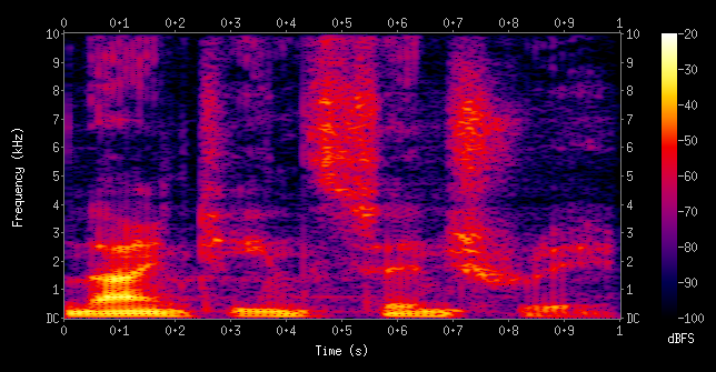 Figure 2: A spectrogram of the spoken words "nineteenth century". X-axis shows time, Y-axis shows frequency, and color intensity represents loudness. [Source: Wikipedia][2]
Anatomy of a Spectrogram
- X-Axis: Time (left to right)
- Y-Axis: Frequency (low at bottom, high at top)
- Color/Brightness: Amplitude (louder = brighter/warmer colors)
Reading a Spectrogram
Once you know what to look for, spectrograms become surprisingly readable:
- Vowels show up as horizontal bands (like stripes)
- Hard consonants ("p", "t", "k") show up as vertical bursts
- Hissing sounds ("s", "sh", "f") show up as fuzzy noise patterns
- Silence shows up as dark gaps
The Crucial Insight for AI
Once we have a spectrogram, speech recognition stops being an "Audio Problem" and becomes a Computer Vision Problem.
The spectrogram is literally a 2D image. We can apply all the techniques that work for image recognition:
- Convolutional Neural Networks
- Pattern matching
- Feature extraction
A Note on Model Architectures: This series focuses on spectrogram-based models like OpenAI's Whisper, Google USM, and Audio Spectrogram Transformers - which treat audio as a 2D "image" of time × frequency. There's also a separate class of waveform models (like Meta's Wav2Vec 2.0 and HuBERT) that process raw audio samples directly, learning their own features rather than relying on human-designed spectrograms. Both approaches have merit, but spectrogram models are currently the dominant architecture for production speech recognition systems.
For spectrogram-based models, a spoken word is effectively just a "shape" on a grid - which is why they can borrow architectures directly from computer vision.
🎹 The Mel Scale: Aligning with Human Perception
We have one more transformation to apply, and it's based on a fascinating fact about human hearing.
Linear Frequency is Not How We Hear
Mathematically, the jump from 100 Hz to 200 Hz is the same as the jump from 10,000 Hz to 10,100 Hz - both are a 100 Hz increase.
But to human ears? The first jump (100→200 Hz) sounds like going up an entire octave (doubling in pitch). The second jump (10,000→10,100 Hz) is barely perceptible.
Our hearing works on a curve, not a straight line. We're super sensitive to small changes in low frequencies (where speech lives) but can barely tell the difference in high frequencies.
The Mel Scale
In 1937, researchers Stevens, Volkmann, and Newman created the Mel scale - a perceptual scale where equal distances represent equal perceived pitch differences.
There's a mathematical formula to convert Hz to Mel, but you don't need to memorize it. Just understand the effect:
| Frequency (Hz) | Mel Value | Perception |
|---|---|---|
| 100 | 150 | Low male voice |
| 500 | 607 | Mid speech range |
| 1000 | 1000 | Reference point |
| 4000 | 2146 | High consonants |
| 8000 | 2840 | Sibilance ("s" sounds) |
Mel Filter Banks: Doing the Warping
To apply this to our spectrogram, we use Mel filter banks - basically a set of "buckets" that group frequencies together.
- Low frequencies (where speech detail matters): Lots of small, precise buckets
- High frequencies (where we just hear "hissing"): Fewer, bigger buckets that average things out

The Log-Mel Spectrogram
The final output is called a Log-Mel Spectrogram:
- Mel-scaled: Frequencies warped to match human perception
- Log-compressed: Amplitudes converted to decibels (log scale), which also matches how we perceive loudness
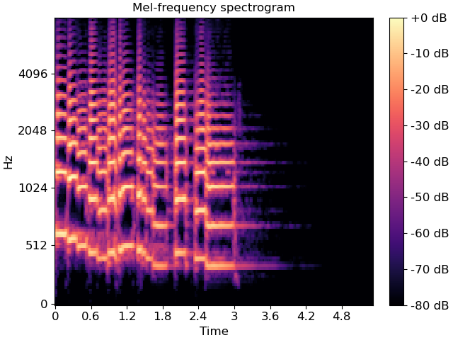 Figure 3: A Mel-frequency spectrogram. Notice how the Y-axis (Hz) is non-linearly spaced - more resolution at lower frequencies where speech detail matters. Compare this to Figure 2's linear frequency axis. [Source: librosa documentation][3]
Why This Matters for AI
The Log-Mel Spectrogram achieves several goals:
- Compression: We go from thousands of frequency bins to ~80 Mel bands
- Perceptual Relevance: We keep detail where humans (and thus training data transcriptions) are sensitive
- Normalized Range: Log scaling keeps values in a reasonable range for neural networks
- Noise Robustness: High-frequency noise gets averaged together rather than dominating
This is the representation that most modern speech AI systems consume.
🔄 The Complete Pipeline: From Air to Array
Let's trace the full journey one more time:

Each step serves a purpose:
| Stage | What It Does | Why It Matters |
|---|---|---|
| Sampling | Converts continuous → discrete | Computers need finite numbers |
| Windowing | Segments time | Captures how speech changes |
| FFT | Reveals frequencies | Exposes the "ingredients" of sound |
| Mel Scaling | Matches human perception | Focuses on what matters for speech |
| Log Compression | Normalizes amplitude | Better range for neural networks |
🎭 Two Philosophies: Spectrograms vs. Raw Waveforms
Before we move on, it's worth acknowledging that the spectrogram approach isn't the only way to process audio for AI. There are actually two major schools of thought:
The "Image" Approach (Spectrogram Models)
Examples: OpenAI Whisper, Google USM, Audio Spectrogram Transformer (AST)
These models convert audio to Log-Mel Spectrograms first, then process the 2D representation:
- Analogy: "Reading sheet music" - looking for visual patterns
- Architecture: Often uses Vision Transformers or CNNs borrowed from computer vision
- Pros: Very efficient; the Mel scale mimics human hearing; well-understood processing pipeline
The "Raw" Approach (Waveform Models)
Examples: Meta's Wav2Vec 2.0, HuBERT, WaveNet
These models skip the spectrogram conversion entirely, ingesting the raw waveform (16,000 numbers per second):
- Analogy: "Feeling the vibration" - learning directly from temporal dynamics
- Architecture: Uses 1D convolutions and sequence models
- Pros: Can learn features that spectrograms might blur out; end-to-end learning
| Feature | Spectrogram Models (e.g., Whisper) | Waveform Models (e.g., Wav2Vec) |
|---|---|---|
| Input | 2D matrix (Time × Frequency) | 1D array (Time × Amplitude) |
| Preprocessing | Human-designed (Mel scale) | Learned features |
| Architecture | Vision Transformers / CNNs | 1D Convolutions / Sequence models |
In this series, we focus on the spectrogram approach because:
- It powers the most widely-deployed models (Whisper, Google's speech APIs)
- The "audio as image" intuition is powerful and accessible
- Understanding the spectrogram pipeline gives you insight into why these models work
But know that the field is evolving, and hybrid approaches are emerging.
🚀 What's Next: Enter the AI
We've traversed the gap between physical reality and digital representation. We started with air pressure variations, digitized them into samples, sliced them into time windows, decomposed them into frequencies, and warped them to match human perception.
The result is a Log-Mel Spectrogram - a compact, perceptually-aligned 2D representation of speech.
But we haven't touched what happens when this "audio image" enters a neural network. How does OpenAI's Whisper model - trained on 680,000 hours of multilingual audio - actually convert these colorful spectrograms into text?
In Part 2, we'll crack open the Whisper model architecture and explore:
- The Encoder: How convolutional layers and Transformers build a "context map" of the audio
- The Decoder: How the auto-regressive text generation actually works
- The Tokenizer: How the model chops words into pieces (and why that matters)
- Multilingual Challenges: Why models sometimes get confused by mixed languages
- Fine-Tuning: How to adapt Whisper for your specific domain
Stay tuned.